Load Balancing Methods

When running dynamic particle simulations on large-scale parallel architectures it is possible that the compute ressources are not utilized in an optimal manner due to different amounts of particles per process that need to be processed or tasks assigned to different processes taking a varying amount of time to be completed. This leads to time spans in which some processes are forced to wait for other processes to complete their work, before the simulation can continue. If these waiting time increase too much, the parallel execution can become very ineffective, as more time is spent waiting on other processes than on actual computation.

There are two different methods to deal with this phenomenon with regard to particle simulations. The first is to design the code in such a way, that in consists of so called tasks, which can shifted from process to process, or thread to thread, depending on the kind of parallelization used. This is called task-based load-balancing. In the SDL Molecular Systems we pursue another technique, which we call geometic load-balancing. In contrast to the task-based load-balancing approach, the code itself is not necessarily design with tasks in mind, but must use domain decomposition as a parallelization strategy. This means that the simulation volume is subdivided into different sub-volumes, which are distributed between the different processes. Due to the dynamic or inhomogenous nature of some particle systems, this might lead to imbalance, as different amounts of particles are assigned to each process. In order to equalize the workload, the shape of the domains are then adjusted to try to compensate these differences, optimally to make these differences disappear, so that waiting times vanish.

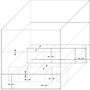
For the geometric load-balancing there are two possible ways, that can be pursued, local and global adjustment. When using local adjustments, only information of a subset of processes, close to each other in space, are used and the domains of these processes are adjusted depending on local workload differences. This leads to iterative types of load-balancing that are suited to be performed during the runtime of simulations, as the overhead is comperatively small. An example for such a scheme can be seen in the scheme on this page, where in a first step the size of process planes are adjusted, then the size of process columns and finally the size of indiviual domainsare adjusted.

In contrast to that, global approaches use all available information in the system to try to compute an distribution of processes, that is as optimal as possible in one step. In comparision to the local approach, usually this leads to a massive redistribution of particles between processes. As a consquence the global approach is more suited for rather static systems that can benefit from a well chosen starting configuration, but do not require an adjustment of domain boundaries during the simulation.

While the task-based load-balancing approaches have their advantages, the SDL pursues the geometric variants, as we think that these methods can be more easily be incorporated into existing codes that might have load-balancing issues, since the only change that needs to be implemented is the ability to be able to deal with changing domain boundaries, which usually is in simple load-balancing schemes not too much of a change in comparision to existing communication schemes.